In July 2017, Stata 15 was officially released. This is the largest version update of Stata ever. We posted the Statalist and listed the 16 most important new features. This article will focus on these new features:
? Extended regression model
? Potential Category Analysis (LCA)
Bayesian prefix instruction
Linear Dynamic Stochastic General Equilibrium (DSGE) Model
? Web dynamic Markdown document
? Nonlinear mixed effect model
? Spatial autoregressive model (SAR)
? Interval censored parameter survival time model
? Finite Mixed Models (FMMs)
? Mixed Logit model
? Nonparametric regression
? Clustering random design and power analysis of regression models
Word and PDF documents
? Graphic color transparency / opacity
? ICD-10-CM/PCS support
? Federal Reserve Economic Data (FRED) support
? Other
Extended regression model
We call this the ERMS extended regression model. Four new commands are suitable
Linear regression analysis,
Interval regression includes the tobit model,
Probability,
Ordered probability model
Can be arbitrarily combined into:
Endogenous variable
Non-random processing tasks
. Selection of endogenous (Heckman-style) samples
These new commands are surprising because endogenous variables can be added to any equation, including processing assignments and probability selection equations. Endogenous variables are not limited to continuity. They can be binary or ordinal. Whether exogenous or endogenous, they can interact with other variables. They can even interact to form a square or cubic term!
These new ERM commands—eregress, eintreg, eprobit, and eoprobit—are destined to be popular because they solve many of the researchers' problems. First, there may be an endogenous variable, because many models omit variables associated with variables in the model. Second, data is often clipped, and clipping is not random. The ERM sample selection option allows you to model and adjust the selection process. Alternatively, if you are using a non-random processing effect model, you can use ERM to handle allocation options. Alternatively, the processing allocation and selection options can be combined, some of which are loss-of-fitting endogenous processing allocation models due to subsequent behavior.
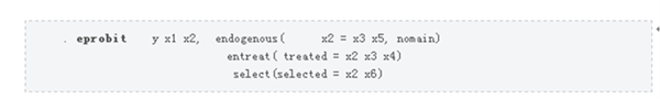
The syntax is very simple:
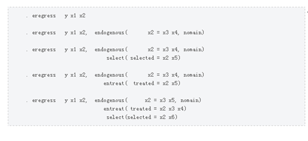
Eregress is suitable for linear regression. The probability model can be easily fitted to a linear regression model. If the resulting variable y is binary, type:
If the resulting variable y is continuous, but the variable x2 is binary, type
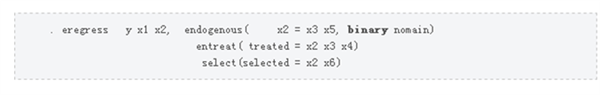
If y and x2 are both binary, type

If you want to know the details of the strange nomain option. When endogenous(name=...) is specified, the variable name is automatically added to the main equation. Can type

or

Either way, the same model is fine. Nomain was specified in the previous example, so I don't need to explain this option including the main equation X2.
2. Potential Category Analysis (LCA)
The potential mean is not observed. Classification is also grouping. Potential classes are groups that are not observed in the data. You may have data about consumers and divide them into three groups based on their potential interest in the product. However, there are no variables in the data that specify the group to which each consumer belongs. If there are four binary variables, they are indications of the potential class to which the consumer belongs, you can type

Y1, y2, y3, and y4 are observed. Consum is a potential categorical variable, and lclass (Consum 3) is specified as a value of 3. The result is a fit of a model where y1, y2, y3, and y4 are determined by unobserved classes. One of the four y variables and one of the three classes, the command is suitable for 4×3 = 12 logistic regression analysis. Each regression has an intercept. In addition, multiple logistic regressions can also be used to predict Consum.
After fitting the model, you can
Use the new estat lcprob command to estimate the proportion of consumers belonging to each category;
Use the new estat lcprob command to estimate the marginal mean of Y1, Y2, Y3, and Y4 in each class (the mean is the probability shown in the example);
Use the new estat lcprob command to evaluate fitness;
Use the existing predict command to get the predicted probability of the classification member and the predicted value of the observed variable.
3. Bayesian prefix instruction
The new bayes: prefix command allows you to adapt to a wider Bayesian model than the previous version. It is also possible to fit Bayesian linear regression, but now you can enter text by:

This is very convenient. Models that fit Bayesian survival cannot be done before. Now you can:

You can even fit a Bayesian multi-level survival model:

In this model, a random intercept is added for each value of the variable id.
The new bayes: prefix command works before many Stata evaluation commands and provides models for more than 50 possibilities. Supported models include multi-level, panel data, survival and sample selection models!
The new command supports the Bayesian functionality of all Stata. You can choose from the distribution of the previous model parameters, or you can use the previous default. When the closed form solution is used in the Gibbs method, the default adaptive Metropolis–Hastings sampling, or Gibbs sampling, or a combination of the two methods can be used. Any other functionality of STATA can be used based on the bayesmh command. You can change the default prior distribution of the regression coefficients, for example, using the prior() option:

After the assessment, you can use the Stata standard Bayesian postestimation tool, such as
Bayesgraph check convergence
Bayesstats summary to estimate the function of model parameters
Bayesstats ic and bayestest model calculate Bayesian factors and compare Bayesian models
Bayestest interval for interval hypothesis testing
4. Linear Dynamic Stochastic General Equilibrium (DSGE) Model
DSGEs ​​are a time series model in economics. They are an alternative to traditional predictive models. Both attempt to explain the general economic phenomenon, but DSGEs ​​allow this to be done on the basis of economic theory models. There are many equations based on economic theory. A key feature of these equations is that the expected value of future variables will affect today's variables. This is a feature that distinguishes DSGEs ​​from vector regression or state space models. Another feature is that the parameters derived from the theory can usually be explained by this theory.
Here is how to fit a two-equation DSGE model in Stata. Braces, {}, used to enclose the parameters:

p is a control variable and y is a state variable in state space terms. f. is the forward operator.
The first equation,

Representing the control variable p depends on the future {beta}*p plus the current {kappa}*y.
The second equation,

The expected future value for y is now {rho}*y. The stata option specifies that y is a state variable.
There are three variables in the DSGE model:
Control variables and equations, such as p, have no impact and are determined by the system of equations.
State variables (such as y) have an implied impact that is predetermined at the beginning of the time period.
Impact is a random error in the drive system.
In any case, the above dsge command can define a model and fit it.
If we have a theory about the relationship between beta and kappa, such as they are equal, we can test it with the existing command test.
The new postestimation commands estat policy and estat transition report policy and transformation matrices. If you type

Displays a linear function that takes a control variable as a state variable. If there are five control variables and three state variables, each control will be reported as a linear function of three states. In the simple example above, the linear function of the predicted p will be displayed as the current y function.
Simultaneously,

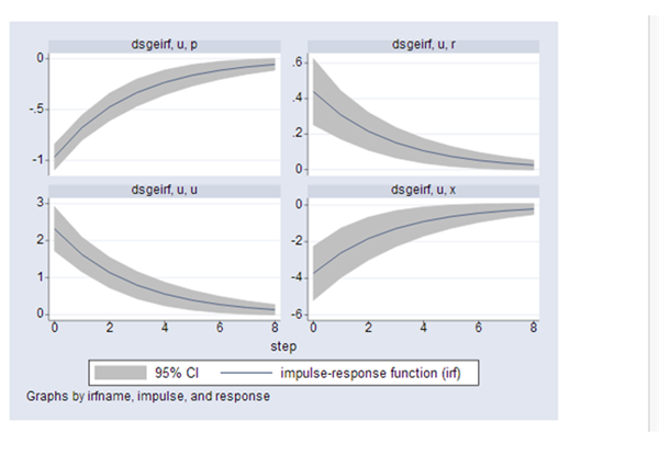
Report the transformation matrix. The policy matrix reports p as function y, and the transformation matrix reports how y evolves into p over time. You can use Stata's existing forecasting commands to generate forecasts. The impulse response function can be drawn using Stata's existing irf command.
This is an impulse response diagram:
5. Web dynamic Markdown document
Have you ever heard of Markdown? It is a popular way to create html documents. The html file is cumbersome. Markdown is simple and intuitive, and the idea is simple. You can create a file that contains the text in the desired readable format and then run a command through it to create an HTML file.
Stata now supports Markdown, we have added tags (features) to Markdown, which allows to include the Stata command in the input file. The commands you include will be run and displayed, or run in secret mode, and extract the output portion for use by the document.
You can create a file, for example
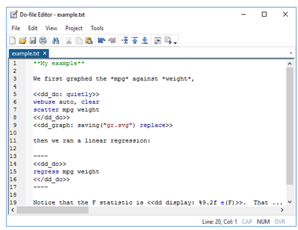
In Stata, you can type

Now, with a new file called example.html, on the web, it looks like this:
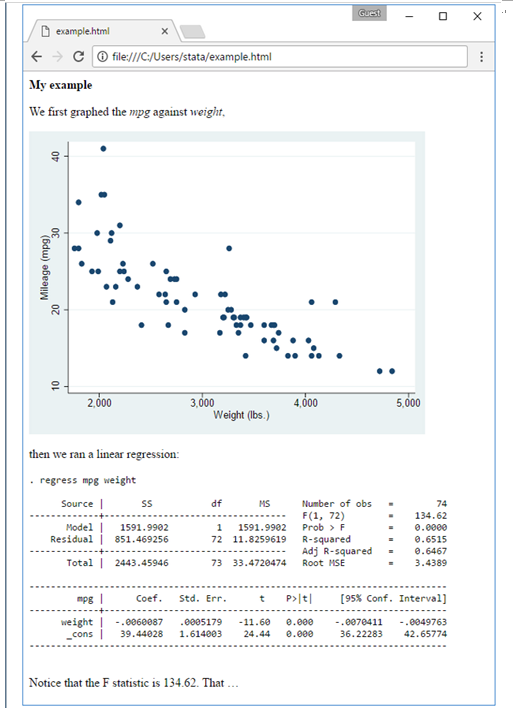
Dyndoc stands for dynamic documentation. The created Markdown file is dynamic. If the data changes, you can recreate the page with a simple input.

6. Nonlinear mixed effect model
Nonlinear mixed-effect models are also known as nonlinear multi-level models and nonlinear hierarchical models. There are two ways to consider these models. Think of them as nonlinear models with random effects. Or they can be viewed as a linear mixed-effects model in which some or all of the fixed and random effects are nonlinear. Either way, the total error distribution is assumed to be a Gaussian distribution.
These models are popular in population pharmacokinetics, bioassays, and research biology and agricultural growth. For example, the drug absorption, seismic intensity and plant growth of the organism were simulated using a nonlinear mixed-effects model.
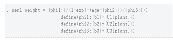
The new evaluation command is named menu. It implements the popular-in-practice Lindstrom–Bates algorithm, which is based on linearization of nonlinear mean functions for fixed and random effects. Supports maximum likelihood and restricted maximum likelihood estimation methods.
Menl is easy to use. You can enter a single equation directly. Braces { } for enclosing the parameters to be matched:

The valuations are b1, b2, and b3. U[plant] is the random intercept of each plant.
Menl can fit a multi-level or multi-level specification where parameters define each level as a model parameter and a random effect function.
This is the same as the previous model. In addition, b2 and b3 allow for changes between different plants. Several variance-covariance structures can be used to model the dependence of random effects at the same level. If you want to model, you can set the dependency in the above example between U1, U2 and U3. Although not explicitly stated, there is an intra-group error in this model. The variance covariance structure is flexibly applied to the modeling of heteroscedasticity and intragroup correlation. Heteroscedasticity can be modeled as a power function of a covariate or predicted mean, and the dependence can be modeled using an autoregressive model of any order.
In addition to the standard functions, the postestimation feature includes predictions of random effects and their standard errors, predictions of parameters of interest defined in the model, parameters of other model parameters and random effects, and overall evaluation of clustering correlation matrices.
7. Spatial autoregressive model (SAR)
Stata is suitable for spatial autoregressive (SAR) models, also known as synchronous autoregressive models. The new spregress, spivregress, and spxtregress commands allow for spatial lag of dependent variables, spatial lag of independent variables, and spatial autoregressive errors. Spatial lag is a spatial simulation of time series lag. Time series lag has become a variable value in recent years. Spatial lag is the value of the nearby area.
This model applies to regional data, also known as regional data. Observations are called spatial units and can be national, state, district, county, city, zip code, or city block, or they may not be geographical at all. They may be nodes of a social network. The spatial model assesses the direct impact—the impact of the region on itself and estimates the indirect or spillover effects of adjacent regions.
There is a new [SP] manual dedicated to Stata's new SAR features. These commands are called Sp commands. They can work with the following:
Shapefiles get your choice data via the web, or
There are no shapefiles and data, only the coordinates of the location, or
• Social network data will appear without a shapefile in place.
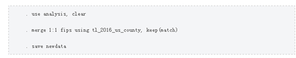
Here's how it works with shapefiles. Visit the US Census Bureau website and download the tl_2016_us_county file. You type now
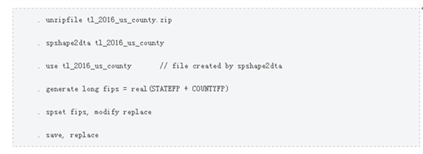
Next, merge the newly created tl_2016_us.county.dta file with your analysis file:
You are ready to define a spatial weighting matrix and a fitted spatial lag model.
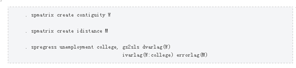
Only fit (1) the spatial lag of the dependent variable of college (2) and (3) the unemployment model of the college space lag. The model also has autoregressive errors. The spatial lag variable is calculated by W, and the spatial lag error is calculated by m.
8. Interval censored parameter survival time model
Stata's new stintreg command is added to streg to fit the parameter survival model. Stintreg fits the interval censored data model. In the interval censored data, the failure time is not determined. As we all know, the subjects have not failed, and when they have failed.
Stintreg fitting index, Weibull, Gompertz, lognormal distribution, logarithmic logic and generalized gamma time-of-flight model. Support for proportional risk and accelerated time to failure metrics. Features include
Hierarchical estimation
Flexible auxiliary parameter modeling
Standard error of robust, cluster–robust, bootstrap, and jackknife
Survey data evaluation is supported by the svy prefix.
In addition to basic functions, the postestimation function includes plots of survivor, hazard, and cumulative hazard functions; mean and median time predictions; Cox–Snell and martingale-like residual values.
9. Finite Mixed Models (FMMs)
New fmm: When the data comes from an unobserved subgroup, the prefix command fits the model. It can be used with 17 Stata evaluation commands.
Most users use fmm to fit the changes in the parameters (coefficient, position, variance, ratio, etc.) in the model between different subgroups. In these models, unobserved subgroups are called classes. For example, the fitting model you are interested in.

But you think that the parameters of the three types of models may be different. Although there is no variable that records class membership, it can be

The report will be three linear regressions—one for each class—along with the model of the predictive class member.
Fmm: When a class may follow different models, you can also use multiple evaluation commands at the same time, such as

In the examples of these two classes, the report will be the first type of linear regression model, the Poisson regression is the second category, and the predictive class member model.
In each proportion of the total population, the Posttestimation command can be used to (1) evaluate, (2) the marginal mean of the outcome variables within the reporting class, and (3) the probability and predictive outcome of the predictive class members.
10. Mixed Logit Model
Stata has fitted multiple logit models. Stata 15 enables them to fit mixed forms, including random coefficients.
Random coefficients have special significance for fitting polynomial logic models. They are a way around the assumption of Independence of the Irrelevant Alternatives (IIA). This assumption suggests that if you choose to walk to work, when your choice is to walk, take a bus, or drive, you still choose to walk, even if you have no option to choose not to reuse. If the option is between walking or driving, you will still choose to walk. Humans sometimes behave differently.
IIA assumes that under the condition of covariates, the choice is independent. If this assumption is violated, the choice will be relevant. The random coefficients allow the correlation to be chosen. Researchers often use hybrid models in random utility models and discrete selection analysis. Stata's new asmixlogit Logit command supports a variety of random coefficient distributions and allows models containing specific case variables.
11. Nonparametric regression
Stata is now suitable for nonparametric regression. In these models, the function form is not specified. Specify variables and specify the variables you want to match:

The match is g(). This method does not assume that g () is linear; it can also

This method does not even assume that g () is linear in the parameters. It can also

For y models of x1, x2, and x3, type

The report is the average of the y partial derivatives, x1, x2 and x3 and standard error. The average is calculated from the data. After fitting the model, predict can be used to obtain the predicted values.
The average derivative is similar to a coefficient, or at least the model is linear, and it is not. Be aware that the average derivative in a nonlinear model is not an average derivative. You may want to know the derivatives of y for x1, x2, and x3 in the mean of the variables. You can get it using margins:

Or, you want to evaluate the predicted value at a specific point of interest,

If you want x3 to be 1, 2,..., 10, you can type

Then you can type

Draw a part of this function.
In addition, margins can not only calculate, but also generate boot standard errors.
12. Power analysis of clustered random design and regression models
Stata's existing power commands perform power and sample (PSS) analysis. Its features include PSS linear regression and cluster random design (CRDs). Now you can add your own power and sample size methods.
New methods for linear regression include
Power oneslope, performs pss on the slope test in a simple linear regression. Calculate the size or power of the sample based on other given research parameters
Power rsquared, PSS performing R-squared test in multiple linear regression. The R-squared test is an f-test for the coefficient of determination (R-squared). Tests can be used to test the meaning of all coefficients, and can also be used to test a subset of them. In both cases, power rsquared calculates sample size or power or target R-squared for other parameters to study.
Power pcorr, performs partial correlation testing of PSS in multiple linear regression. The partial correlation test is a test of the square-biased multi-correlation coefficient f. This command calculates the sample size or power or target squared partial correlation coefficient based on other research parameters.
Stata 15 now also supports cluster randomization:
In the CRD, the subjects (clusters) in the group are random rather than individual, which means that the size of the sample is played through the size of the cluster and cluster size. The sample size determines the number of given cluster sizes or the size of a given cluster. The CRD command calculates (1) the number of clusters, (2) the cluster size, or (3) the power, or the minimum detectable effect size given by other parameters. These commands can adjust options based on unequal cluster sizes.
When specifying a new option cluster, the existing 5 power methods will be extended to support CRDs. They are
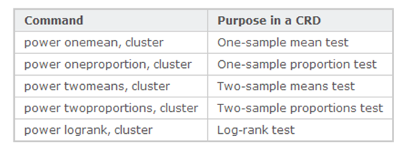
For two sample methods, you can also adjust for unequal clusters in both groups.
Like all other power methods, the new method allows multiple parameter values ​​to be specified and automatically generates table and graph results.
Another new feature is the ability to add your own PSS method. This is very easy to do. Write a program that calculates the sample size, power, or effect size. The power command will do the rest for you. It handles the support of multiple values ​​in options and automatically generates graphs and result tables.
13. Word and PDF documents
Now, using the results of Stata embedding to generate Word and PDF files is as easy as creating an Excel worksheet. Most users like putexcel in Stata 14, and if you are one of them, you will fall in love with the new putpdf and putdocx commands. They work like putexce. You can write a do-file to create an entire Word or PDF report with the latest results, tables, and charts. Repeatable reporting can be performed automatically.
The new putdocx command writes paragraphs, images, and tables to a word document (.docx file). Images include Stata graphics and organizational logos. You can also format the text object. Includes font size, bold, skew, custom tables, and more.
14. Graphic color transparency / opacity
Up to now, draw an object on top of the other, and the object above covers the object below. In the jargon of computer graphics, the Stata color is completely opaque, or, if you prefer, it is not completely transparent. Stata 15 allows to control the opacity of its color.
The opacity is specified as a percentage. By default, Stata's color is 100% opaque.
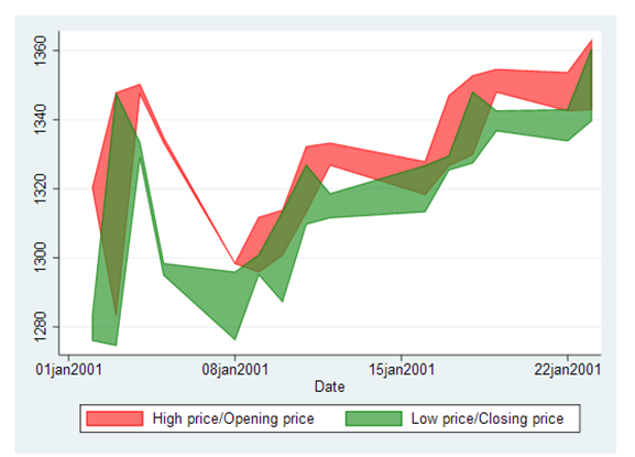
You can specify opacity whenever you specify a color, such as controlling the color of a marker in the mcolor () option. You can specify green%50 instead of green. You can specify "0 255 0%50" instead of "0 255 0%50" (equivalent to green). You can specify %50 by yourself to make the default color 50% opaque. However, do not specify %0. This is completely transparent and intangible.
Here is a chart that uses 70% opacity:
15. ICD-10-CM/PCS support
Stata 15 supports ICD-10-CM and ICD-10-PCS, the US ICD-10 code provided by NCHS and CMS. Stata 15 supports code starting with the 2016 release (starting October 2015), when they are licensed for use in the US, and supports all subsequent releases.
Stata began supporting ICD in 1998, starting with the ICD-9-CM 16 release and supporting each subsequent ICD-9 release. Since 2003, Stata has also supported the ICD-10 code version.
Since 1998, Stata's ICD commands have been just an automatic list of valid codes and short phrases, becoming the entire data management system for ICD code. The system even includes the ability to manage multiple ICD versions in one data set!
16. Federal Reserve Economic Data (FRED) support
The St. Louis Federal Reserve provides more than 470,000 US and international economic and financial time series to registered users. Registration is free and easy to do. This service is called FRED. It includes data from 84 sources, including the Federal Reserve, the Pennsylvania World Table, Eurostat and the World Bank.
In Stata 15, you can use Stata's GUI to access and download FRED data. You can search or browse by category, release, or source. You can click to select the series of interest. Choose 1 or choose 100. When you click Download, Stata will download them and merge them into a single custom data set in memory.
The Stata command line interface also provides these same features. The command is import fred. This command is very convenient when tracking monthly reports requires automatic updating of 27 different series.
Stata has access to FRED and ALFRED. ALFRED is the historical archive data of FRED.
17. Other
Learn more about these features in the Stata Features page, as well as the following features:
Bayesian multi-level model
Threshold regression
. Panel data tobit with random coefficients
Multi-layer regression of interval measurement results
Multi-level Tobit regression of censored results
Cointegration test of panel data
Multi-breakpoint test in time series
Multiple sets of generalized SEM
Linear regression of heteroscedasticity
Heckman-style sample selection Poisson model
. Panel data nonlinear model with random coefficients
Bayesian panel data model
. Panel data interval regression with random coefficients
. SVG export
Bayesian survival model
Zero expansion ordered probability
. Add your own power and sample size methods
Bayesian sample selection model
. Support Swedish
. Improvements to the DO file editor
Stream random number generator
Improvements to the java plugin
Stata / MP more parallelization
This Upholstered Chair is very popular and widely used in home, coffee shop and restaurant, you could match our Home Table together.
We use environmental material and provide the perfect replica items.
pp seat inside and we upholstery the patchwork ourside, and also we have many colors to choose.
To provide you the best craft is our purpose.
We also have many Home Accessories to decorate your home.
If you need more information, just feel free to contact me, I will send you more details pictures and information.
Upholstered Chair,Eames Patchwork Chair,Eames Upholstered Chair,Dar Patchwork Chair
Ningbo Realever Enterprise Limited , https://www.realeverfurnishing.com